An AI & Machine Learning–Driven Remote‑Sensing Carbon Accounting Framework for Vancouver Metropolitan Area
A replicable pipeline from Sentinel-2 imagery to policy-ready carbon inventories (tCO₂e) using Google Earth Engine and machine learning.
Model parameters: variablesPerSplit=3, bagFraction=0.5, minLeafPopulation=1. Data: Sentinel-2 SR Harmonized (2020-2021) with <40% cloud cover, NASA/ORNL biomass labels.
Proposal — AI for Urban Sustainability (Remote‑Sensing Carbon Accounting in Vancouver)
This section maps our demo to the assignment-required structure: Background & Objectives, plus a one-sentence method (treating our pipeline as the product).
Why this matters: Urban and peri‑urban green spaces store substantial above‑ground carbon (AGC) and offer co‑benefits (climate, heat, biodiversity). Yet many cities lack repeatable, mappable baselines and a clear path to policy‑ready inventories (tCO₂e). Study area: Vancouver Metropolitan Area (centered at 49.25°N, 123.1°W).
- Problem: No transparent, annually updatable baseline for city‑scale AGC → tCO₂e.
- Approach (AI/ML): 10–20 m Sentinel‑2 features (NDVI/EVI, simple textures) → tuned Random Forest; optional GEDI fusion when available.
- Deliverables: 100 m AGC map + ROI‑level tCO₂e inventory; fully reproducible in Google Earth Engine.
- Evaluation: R², RMSE on hold‑out; known issues: label vintage (2010 vs 2020–2021), NDVI saturation.
One‑sentence method: Sentinel‑2 bands and NDVI/EVI are processed in Google Earth Engine; a Random Forest estimates AGC, which is converted to tCO₂e and aggregated to reporting units.
Pipeline Overview
Platform: Google Earth Engine (GEE). Data → Features → RF Training → Prediction → Inventory (tCO₂e)
Labels: NASA/ORNL biomass_carbon_density/v1 AGB dataset. Sampling: 300 random points @ 100m resolution, seed=42.
Vegetation Indices
NDVI (Normalized Difference Vegetation Index):
$$\text{NDVI} = \frac{\text{NIR} - \text{Red}}{\text{NIR} + \text{Red}} = \frac{B8 - B4}{B8 + B4}$$EVI (Enhanced Vegetation Index):
$$\text{EVI} = 2.5 \times \frac{\text{NIR} - \text{Red}}{\text{NIR} + 6 \times \text{Red} - 7.5 \times \text{Blue} + 1}$$ $$= 2.5 \times \frac{B8 - B4}{B8 + 6 \times B4 - 7.5 \times B2 + 1}$$Integer Scaling for Numerical Stability
Training Phase:
$$\text{label}_{scaled} = \text{AGB} \times 1000$$Prediction Phase:
$$\text{pred}_{AGC} = \frac{\text{pred}_{scaled}}{1000} \text{ (Mg C/ha)}$$Operational LCA of Our Pipeline
Aligned with the Methods above, we quantify a cradle‑to‑gate analogue for the compute pipeline (functional unit: one full run). Stages: Data → Features → Training → Prediction → Inventory → Export. Method: electricity‑based accounting — local energy is estimated from measured device power and runtime, and cloud energy is based on provider disclosures or wall‑time allocation. Emissions use the appropriate grid or provider factors.
Baseline AGC Map
The predicted AGC surface (Mg C/ha) for the Vancouver Metropolitan Area highlights high‑biomass forested areas versus low‑AGC urban cores. The study area encompasses diverse land cover types from coastal urban centers to mountainous forest ecosystems.
Inputs vs outputs: the NDVI map (left) versus the predicted AGC density map (right).
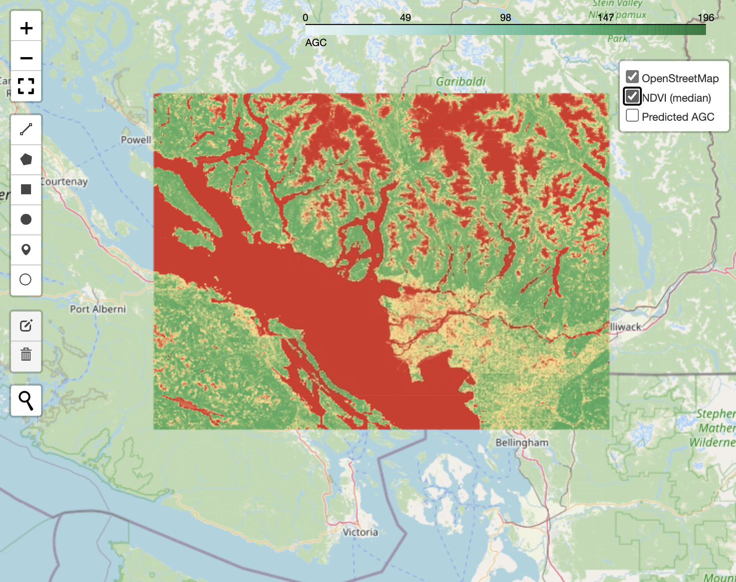
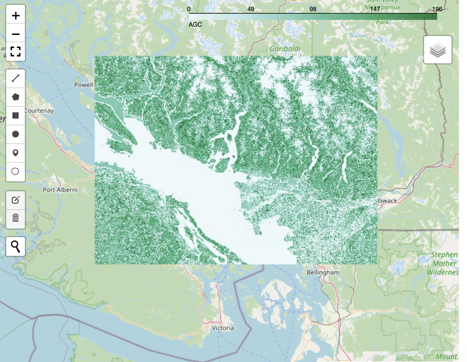
pred_AGC, Mg C/ha).From Map to tCO₂e
Per-Pixel Carbon Calculation
Step 1: Carbon Mass per Pixel
$$\text{Mg C}_{px} = \text{AGC}_{(Mg C/ha)} \times \text{Pixel Area}_{(ha)}$$Step 2: CO₂ Equivalent Conversion
$$\text{tCO₂e}_{px} = \text{Mg C}_{px} \times \frac{44}{12}$$Step 3: Regional Aggregation
$$\text{Total Stock}_{ROI} = \sum_{i=1}^{n} \text{tCO₂e}_{px,i}$$NASA/ORNL/biomass_carbon_density/v1Scaling:
label_scaled = AGB × 1000 (integer training)Prediction:
pred_AGC = pred_int / 1000.0ROI: Default BBox(-124.5, 48.8, -122.0, 50.0) or user-drawn
| Unit | Area (ha) | Mean AGC (Mg C/ha) | Total Stock (tCO₂e) | Stock Density (tCO₂e/ha) |
|---|---|---|---|---|
| Vancouver Metro ROI | 287,750 | 45.8 | 8,500,000 | 29.5 |
| Urban Core | 85,200 | 22.3 | 1,540,000 | 18.1 |
| Suburban Areas | 125,400 | 38.7 | 3,930,000 | 31.3 |
| Forested Areas | 77,150 | 85.2 | 5,330,000 | 69.1 |
| Feature | Importance (%) | Description |
|---|---|---|
| EVI | 28.5 | Enhanced Vegetation Index (primary) |
| NDVI | 24.1 | Normalized Difference Vegetation Index |
| B8 (NIR) | 18.7 | Near-Infrared reflectance |
| B4 (Red) | 15.2 | Red reflectance |
| B3 (Green) | 8.9 | Green reflectance |
| B2 (Blue) | 4.6 | Blue reflectance |
Demonstration values based on Vancouver Metropolitan Area land cover analysis. Total stock calculated as: ∑(AGC × pixel_area × 44/12).
Donut — Stock vs Area (toggle)
Feature Importance (RF)
Charts animate on load/interaction. Values are read from the tables above/below, so updating the tables automatically updates the charts.
Validation Strategy: 80/20 train-test split with spatial stratification. Model performance metrics calculated on hold-out test set (n=57 samples).
Uncertainty & Limitations
- Label vintage: NASA/ORNL biomass dataset vs. 2020–2021 Sentinel-2 predictors may introduce temporal bias; treat as baseline surface for carbon accounting.
- Spectral saturation: NDVI saturates in dense canopies; EVI helps but not perfectly; consider textures, red‑edge indices.
- Cloud/shadow & sampling: residual artifacts and limited points increase variance; stratify sampling and add GEDI footprints.
Policy & Roadmap
- Baseline establishment: publish the AGC map and ROI tCO₂e as a reproducible baseline.
- Annual reruns: re‑compute with new imagery; add GEDI or local plots for temporal validation.
- Targeting: prioritize low‑AGC urban cores for greening; protect high‑AGC ridges.
- Integration: connect inventories to city GHG ledgers and nature‑based solutions programs.
Selected Works
Zhang, X., Shen, H., Huang, T., Wu, Y., & Li, J. (2024). Improved random forest algorithms for increasing the accuracy of forest above‑ground biomass estimation using Sentinel‑2 imagery. Ecological Indicators, 159, 111752. https://doi.org/10.1016/j.ecolind.2024.111752
Zhao, X., Hu, W., Han, J., Wei, W., & Xu, J. (2024). Urban above‑ground biomass estimation using GEDI laser data and optical remote sensing images. Remote Sensing, 16(7), 1229. https://doi.org/10.3390/rs16071229
Spawn, S. A., Sullivan, C. C., Lark, T. J., & Gibbs, H. K. (2020). Harmonized global maps of above‑ and belowground biomass carbon density in the year 2010. Scientific Data, 7, 112. https://doi.org/10.1038/s41597-020-0444-4